The Naïve Bayes Algorithm

In this post we explain how the supervised machine learning technique of the Naïve Bayes Algorithm works when applied to the classification of documents.

Classifying Documents

So far, in the previous blog posts, we have seen how we can determine what are the important phrases of a document and what phrases make it stand out from other documents using tf-idf. We then saw how to use the results of tf-idf to compare one document to another to determine how similar the documents are using the cosine of the angle between the tf-idf vectors of documents we want to compare. We just finished looking at how we can use the tf-idf vectors to create groupings of many documents into the most diverse groups possible using the K-means method. So, what is next?

(If you are thinking what the K-means are you tf-idf talking about, please go back and read the previous three articles)

We will extract factors from the document and then classify the document based on those factors with a Naïve Bayes machine learning algorithm. This article will be a little longer than the others so get comfortable and take a relaxing breath. Just like what we saw in the K-means article we use fancy math, Naïve Bayes, to provide the machine learning capability.

Unlike K-means which is an unsupervised machine learning algorithm, we just handed it our data and it did its thing, Naïve Bayes is a supervised learning algorithm. This means we must train the algorithm with data that we know what the answer should be. Let us get started with the creation of the training data.

Simplifying with Factors

Our first step is to turn a huge amount of data into a handful of factors that we can work with. I know that there are those who would say load everything into the computer and let it figure it out. That is not our approach, we model our systems along the lines of how humans approach things, with context.

When someone says ‘hand me a book’ you would generally not consider the weight of the book when selecting it. You would probably think about what authors the person might like, how long is the book, what is it about, etcetera.

However, if the person was staring menacingly at a great big bug when they said ‘hand me a book’ you might consider how heavy is the book and is it one that no one would ever want to read again when making your selection.

Thus, context would impact what data we would consider when making a decision. This is one aspect of creating factors, filtering data based on the context of the situation.

A second aspect of creating factors is reducing the amount of data by grouping data points. In our book example we could group, number of pages, and font size when determining how long it would take to read a book. Yes, we could use the number of words to determine how long it would take to read a book.

That data is independent of page count and font size however most books don’t tell you the number of words. That piece of data is not available without considerable work, and you really don’t need that level of detail to make your decision. We might group font and page count into a factor called reading length, with a large font and a lot of pages and normal font and fewer pages both having the value of acceptable length.

When selecting a book we might use factors like is it one of our favorite authors, is it an acceptable length, did my friend read it and they liked it, etcetera. So rather than use all the data available to us regarding an array of books, we filter and group the data into a smaller number of factors that will allow us to handle the decision of selecting from an array of books.

Selecting Based on Probability

We see a book that is by an author we like, and our friend read it and said she liked it, and it is on sale for half price. It might be worth buying. It is not a guarantee. Remember when our favorite mystery author tried to write a romance, not good. Remember that one book our friend liked, that was terrible, I can’t believe she liked it. Finally, we don’t have great luck buying books on sale, but there was that one book, and it was great. Will I like it if I buy it?

Essentially that is how the Naïve Bayes algorithm works. It takes the probabilities of various factors and based on what those factors are, determines the likely outcome. Most of the time we like books by authors we like, most of the time we like books our friend likes, but most of the time we don’t like bargain priced books. Should I classify this book as worth the price and buy it.

Great but how can we make a computer ‘think’ like that using the fancy math in the Naïve Bayes algorithm? That is the next part of this article.

Machine Learning Is Just Math

The equation of Naïve Bayes is shown in below.

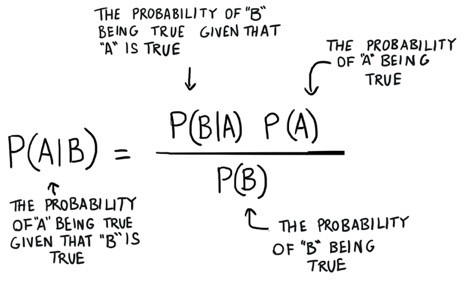
This looks a little scary, but it is straight forward. In words this equation is saying: The probability of A occurring given we see B is equal to the probability of B occurring, given we see A multiplied by the probability that A might occur regardless of B being there or not, all divided by the probability that B might occur regardless of A being there or not. Still confused? Let us turn back to the book example.

The equation below adds in book example labels for me liking a book when my friend likes a book. In words, this equation says “the probability of me liking a book my friend likes, is equal to the probability of my friend liking a book I like, times the probability of me liking a book all divided by the probability of my friend liking a book”.

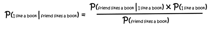
Using numbers, if I like only some of the half price books I buy (30%), and my friend likes most of the books she reads (80%) and my friend likes almost all of the books I recommend to her (90%), then the chance I will like a book she likes is (90% x 30%) ÷ 80% = 33%. So, if our friend likes the book on sale that improves the likelihood, I will like it as well, but just by a little bit.

Now what about the fact it is by an author that we like. How do we add that into the equation? Well it is just another condition added to the probability. The equation would look like the one shown in below

If I like most of the books written by authors I like (80%) and that half of the books I read are by authors I like (50%) I can now calculate the probability that I will like the book that is on sale that my friend likes and is by an author I like.

The answer is: (90% x 80% x 30%) ÷ (80% x 50%) = 54%.

Given there is better than a 50% chance that I will like the book, I think I will buy it.

Okay but where does the Naïve part of Naïve Bayes come from. That is a little more complicated, but it refers to the fact we are assuming that whether our friend likes a book or whether we like the author are completely unrelated. It is a weak assumption that the author plays no role in whether I or my friend like the same book. It may play a significant role in whether we like the same book. To ignore this potential connection between two factors that we are using is said to be naïve. Much analysis has been done to determine if this naïve assumption of factor independence would eliminate the effectiveness of using the Bayes algorithm and the result has been, no it does not eliminate the effectiveness. Naïve Bayes does work.

Where is the learning?

The above discussion has explained how the Naïve Bayes algorithm can be used to classify a document into the groups of, I will like it, and I will not like it. What we have not shown is how this algorithm learns. How does it improve over time and adapt to new information? The answer is in the probabilities. In the above example we said, “I like most of the books written by authors I like” and we assigned a probability of (80%). How did we know that?

That answer is data we collect and store. Imagine that every time you bought and read a book, you kept a simple diary. In it you wrote the author, whether your friend has read it and liked it, whether you bought it on sale and whether you liked it. Over time you would generate a history of data that has the factors friend likes or doesn’t, author liked or not, and bought on sale or not, matched with the outcome of you liked it or you did not.

We use this data to create the probabilities that we used in the above equations. We also use this data to test whether those probabilities are useful. If we have 200 entries in our diary which gave the above probabilities that we used in the equations, we would say that the Naïve Bayes Classifier was trained using that data set. The classifier ‘learned’ from our past experiences displayed in the training data set.

Let’s assume that we bought that book from the bargain table and it was terrible. We would add that data to the diary and the probabilities would be adjusted, in this case lowered. The percentage of books that our friend likes, and I like would be reduced, the probability that I like the author would be reduced and the probability that I like a bargain book would be reduced. Now imagine over a year that we enter information for 100 books that we bought under many different circumstances, some on sale, some by authors I like, some are books my friend likes etcetera. After this new data is used to calculate probabilities perhaps, we find:

We do like most of the books written by authors we like (80%) We do like almost all of the books our friend likes (90%) But we have learned the probability of liking a bargain book is low (10%) So now when confronted with the question of should we buy the bargain book, that our friend likes, by an author we like, we have learned the likelihood of us enjoying the book is low at a level of (90% x 80% x 10%) ÷ (80% x 50%) = 23%. So, unless it is a total steal, it probably isn’t worth it for us to buy it.

To Sum Things Up

This was interesting, and we took you along on a little journey from using tf-idf and cosine similarity to determine similar documents, to using K-means to help group documents, to now using Naïve Bayes to classify the documents. You may be asking please sum this up because it has been a bit of a winding road.

We use the Naïve Bayes Classifier to assign documents describing Intellectual Property that we are interested in to a group which would denote the quality of the intellectual property. We do this by gathering a whole bunch of documents that describe intellectual property and are a member of a known category. An example would be, heavily litigated patents that were upheld by the courts. We extract meaningful factors from this collection of documents and create a data set. This data is used to train a classifier. We then test the classifier using additional data that we gathered.

Just like the book example above as the data set grows the classifier learns and improves in assigning a document to a classification group.